Crescent-1
A Data Science tool for construction companies. Uses Multiple Linear Regression to predict profits based on suppliers, location, sq. footage, etc. Processing and analysis optimized by the Gradient Descent Algorithm. Built in Python.


What It Is
Crescent-1 is a Data Analytics tool for construction companies. It helps make data-driven business decisions by finding patterns in historical data. It can, for example, be used to predict profits for an upcoming year depending on several criteria such as house type, location, time of year, square footage, etc. It reconciles all these criteria statistically and comes up with a prediction model, that can then be used to predict profits for a particular year. It can be further utilized to predict other useful data like location with most sales, most sold type of house, material that contributes the most to losses, etc. This is how Crescent-1 can help you make smart decisions that result in better outcomes for your business.
Installation
Crescent-1 requires Python3 and MySQL Server from Oracle to be installed in the system. This program is made to work on a local sql database for ease of testing. You can choose to use MySQLWorkBench if you prefer executing the queries manually instead of SetupSQL.py. The queries are present under the sql folder.
Note: Oracle’s MySQL database usually reads from port 3306.
Installing Python3 in your system will also install pip in your system, which is a package manager for python.
Install mysql-connector-python
> pip install mysql-connector-python
Install Numpy
> pip install numpy
Install matplotlib
> pip install matplotlib
Next, setup the database connection settings in queries.py inside initSQL() function. The code looks like this:
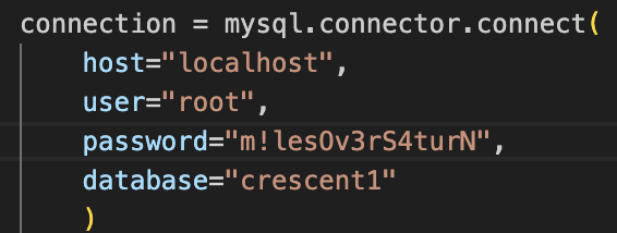
You can choose to setup your database with these credentials, or change it to suit your needs.
Now, we are ready to run the scripts. Refer to Usage to read what each of the scripts do.
Usage
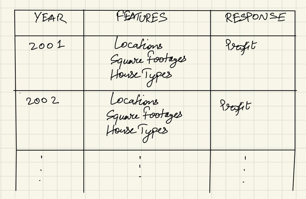
The first step to using this tool is to make a list of features for your problem. A feature is a variable that is independent from everything else in the dataset, but still contributes to change in the final resultant value. It is also called an independent variable. Taking the example of calculating profits from selling houses, the features in this case would be location, house type and square footage.

Next, we need the historical data. This would be the data that has feature values and their corresponding profit numbers on a per-year basis. After feeding this dataset to the program, it closely predicts a new profit number based on a new set of feature values provided by the user.
Running this program without a dataset is also possible. Using dataGenerator.py, one can create mock data just for the purpose of testing this program. This script generates a list of CSV files which can then be fed into another script called SetupSQL.py which then parses and populates an SQL database. Lastly, the script ML.py reads the tables, modifies the data to make it ready for MLR, then runs the algorithm. It then asks the user to enter a set of values for making a prediction. That’s how one can predict profit numbers with the data they have.
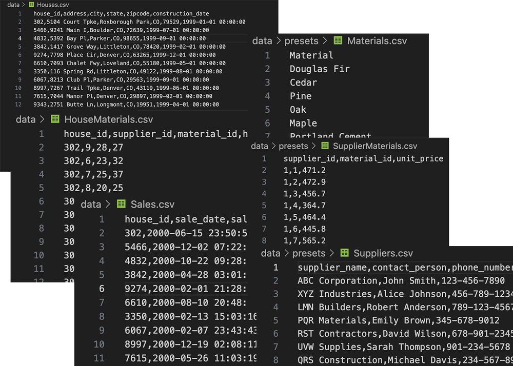
The output files of dataGenerator.py
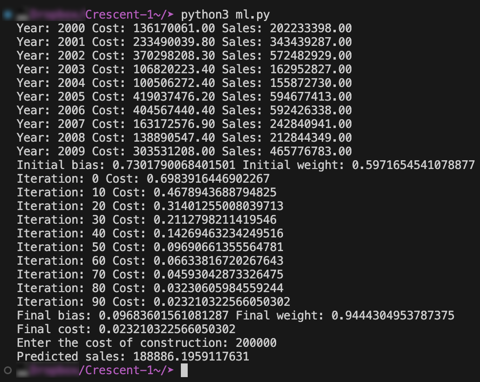
ML.py
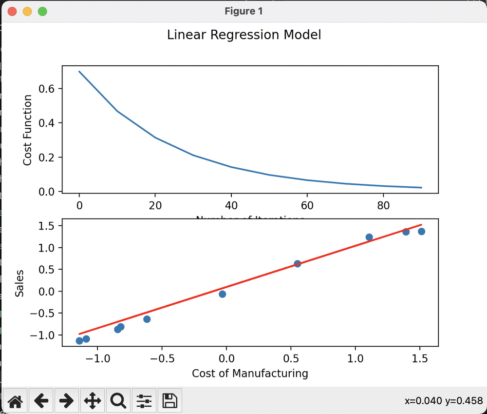
ML.py also outputs a graph that shows the progress of the cost function and the training dataset
How it works
In order to explain how this program works, we need to first talk about Multiple Linear Regression and Gradient Descent.
Multiple Linear Regression (MLR) is a statistical technique used to model the relationship between a single dependent variable (profit) and two or more independent variables (location, type, sq.ft). The independent variables are called features, and the dependent variable is called the response. The goal is to understand how the features collectively influence the response value and to predict the value of the response based on the values of the features.
The dataset used to train MLR in this program is temporal. For example, for a set of data for 5 years, every single year has its own feature values and its own response value. If we take the example of the features from above such as location, type and sq.ft., each year contains its own value for location, type and sq.ft. along with the profit for that year. MLR looks at these features vs response relationships in a per-year basis, then it predicts a new response value for a new set of feature values entered by the user. For example, now we can find the profit that we might get for a house made in Denver that is a two-story with 1200 square footage of area.
Gradient Descent (GD) is a technique that iteratively regresses the cost function towards its most minimum value and is an alternative way of implementing and optimizing MLR. A cost function is a value that gauges how accurate the prediction model is compared to the training dataset. By minimizing this value as much as possible, the algorithm gets closer to finding the best bias and weight values, that makes the prediction model more accurate. One big advantage of using GD is it provides better performance when dealing with large datasets.
We also make use of the equation used to represent straight lines, as in y = mx + c. Here, m is the slope and c in the y-intercept. Multiplying an x coordinate by the slope, and adding the y-intercept yields its corresponding y coordinate. In MLR, the slope is the weight and the y-intercept is the bias. The MLR equation looks as follows:

Here, beta-0 is the bias (or y-intercept) and [beta-1 … beta-n] are the weights. The only difference between this and the equation for a straight line is that there is only one y-intercept value, but multiple weights that each act as a coefficient to their respective feature values. Y-hat represents the predicted response values for each set of feature. The feature values are represented by X1 for feature1, X2 for feature2 and so on. X1 is not a single value, but a list of values for that particular feature. And its coefficient (beta-1) is not a single value, but a list coefficients each corresponding to their respective X1 values. So, X1 is a list of values for feature1 such as location, X2 is a list of values for feature2 such as type of house, and so on.
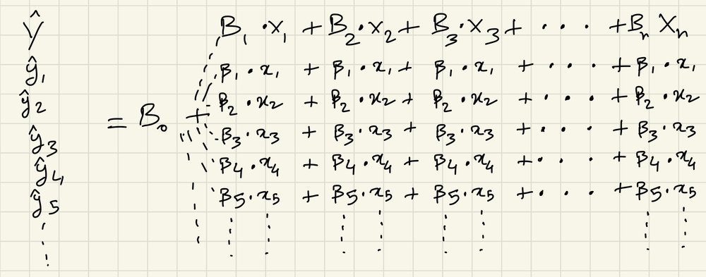
We will call this our prediction equation
Now, we are ready to run MLR in conjunction with GD. First, the bias and weights are initialized to anything random. This bias and weight is fed to the prediction equation to yield Y-hat. Note that we have Y, a list of response values from our training dataset. We feed Y-hat and Y into our cost function:

We are currently inside an iteration of GD. If iteration isn’t complete yet, we use these next set of equations to calculate new bias and weight values.


Alpha is the learning-rate, which defines the incremental rate of the values during each iteration. After this, we go back to step 1 where these new bias and weights will be fed into the prediction equation once more. The number of iterations of GD is a user defined value so here we choose to run 100 iterations. The cost function gradually gets minimized through the process, and after the iteration is complete, the final bias and weight values are what we use later for our prediction.
Let’s say we have houses we plan to sell in a particular year. We first need the list of houses each with their built location, area in square footage and their type. Next, we organize our data in order to feed it to the program. X1 is the list of locations of each house, X2 is the list of square footages of each house, and X3 is the type of each house. We have the bias and weight values from our MLR above. We plug all of these values into our prediction equation, and the response value we get is the predicted profit that we might make on these sales.
